Disclaimer: This post is part of a series about Noncommutative Geometry. I do not pretend to be rigorous nor thorough. The main idea is just to cover (in a rather informal way) the main concepts.
The fuzzy sphere is a really nice example of how the Noncommutative Gel’fand-Naimark Theorem (NCGNT) can be used to define Noncomutative Geometry (NCG) in terms of a Noncommutative Algebra (NCA). Now we will talk about how Alain Connes deepened the understanding in this correspondence. Before doing that, we would like to point out that Connes did not share the motivation of the physicists we mentioned in the previous entry. In other words, his principal motivation was not the geometric measurement problem, he actually wanted to write the distance function in algebraic terms. This might sound easy, but believe me, it is not an easy task at all. For the rest of this post, we will introduce something known as spectral calculus, which is the generalisation of ordinary calculus. Turns out that in order to do this, we also need to define the noncommutative generalisation of a distance function, thus obtaining for free spectral geometry.
Let us start by fixing a Hilbert space 
Suppose that 


Definition 1 Letand
be the eigenvalues of
, if
Then we say that
.

Next, we want to define a differential 
where 

![{[F,a]\in \mathscr{K}(\mathscr{H})}](https://s0.wp.com/latex.php?latex=%7B%5BF%2Ca%5D%5Cin+%5Cmathscr%7BK%7D%28%5Cmathscr%7BH%7D%29%7D&bg=ffffff&fg=000000&s=0&c=20201002)

![\displaystyle da=[F,a]\qquad ( \text{ for all }a\in \mathscr{A}), \ \ \ \ \ (2)](https://s0.wp.com/latex.php?latex=%5Cdisplaystyle+da%3D%5BF%2Ca%5D%5Cqquad+%28+%5Ctext%7B+for+all+%7Da%5Cin+%5Cmathscr%7BA%7D%29%2C+%5C+%5C+%5C+%5C+%5C+%282%29&bg=ffffff&fg=000000&s=0&c=20201002)
Definition 2 (Fredholm module) An odd Fredholm module overAn even Fredholm module is given as above plus a
- An involutive representation
of
- An
,
s.t.
for all
grading
,
s.t.
.
Let us now introduce a fundamental concept if we are intending to do NCG (or any geometry for that matter), the distance.
Definition 3 Letbe the line element for a Riemannian manifold
, then the geodesic distance between
and
is given by

A generalisation of this is given by introducing the “baby steps” operator
Definition 4 Let
we note that
is a positive infinitesimal, from which we can make the association
. Furthermore, we demand that
![{[g,F]=0.}](https://s0.wp.com/latex.php?latex=%7B%5Bg%2CF%5D%3D0.%7D&bg=ffffff&fg=000000&s=0&c=20201002)
![\displaystyle \mathscr{K}\ni g=(dx^\mu)^*g_{\mu\nu}dx^\nu=([F,x^\mu])^*g_{\mu\nu}[F,x^\nu], \ \ \ \ \ (4)](https://s0.wp.com/latex.php?latex=%5Cdisplaystyle++%09%09%09%5Cmathscr%7BK%7D%5Cni+g%3D%28dx%5E%5Cmu%29%5E%2Ag_%7B%5Cmu%5Cnu%7Ddx%5E%5Cnu%3D%28%5BF%2Cx%5E%5Cmu%5D%29%5E%2Ag_%7B%5Cmu%5Cnu%7D%5BF%2Cx%5E%5Cnu%5D%2C+%09%5C+%5C+%5C+%5C+%5C+%284%29&bg=ffffff&fg=000000&s=0&c=20201002)
As we mentioned at the beginning of this post, one of the main objectives of Connes was to write the distance function (3) in purely algebraic terms. This can be done if we replace the points 


We note that we can write ![{df/ds=[F/g^{1/2},a]}](https://s0.wp.com/latex.php?latex=%7Bdf%2Fds%3D%5BF%2Fg%5E%7B1%2F2%7D%2Ca%5D%7D&bg=ffffff&fg=000000&s=0&c=20201002)
![\displaystyle d(\phi,\xi)=\sup \{|\phi(f)-\xi(f)|: f\in \mathscr{A}, \big|\big|[Fg^{-1/2},f]\big|\big|\leq 1 \} \ \ \ \ \ (6)](https://s0.wp.com/latex.php?latex=%5Cdisplaystyle+d%28%5Cphi%2C%5Cxi%29%3D%5Csup+%5C%7B%7C%5Cphi%28f%29-%5Cxi%28f%29%7C%3A+f%5Cin+%5Cmathscr%7BA%7D%2C+%5Cbig%7C%5Cbig%7C%5BFg%5E%7B-1%2F2%7D%2Cf%5D%5Cbig%7C%5Cbig%7C%5Cleq+1+%5C%7D+%5C+%5C+%5C+%5C+%5C+%286%29&bg=ffffff&fg=000000&s=0&c=20201002)
Which suggests introducing the operator
also known as the Dirac operator. Therefore, if we wish to define distance in algebraic terms, we need to prescribe an algebra 


Let us continue, we will say that the triple is of dimension 


Definition 5 (Dixmier Trace)In analogy to the trace, it is linear
for complex
. It is cyclic
if
is bounded. And
when the order of
, as we wanted.

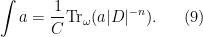
Then, using this and the data provided by the spectral triple, we define:
Definition 6 (Spectral integral) For aWhere
is just to guarantee scale independence, futhermore, we guarantee tameness by imposing
.
All of the above is summarised in the following table
| Commutative | Noncommutative |
| Complex variable | Operator in |
| Real variable | Self-adjoint operator in |
| Infinitesimal | Compact operator in |
| Infinitesimal of order | Compact operator whose eigenvalues decrease as 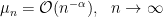 |
| Differential | ![{da=[F,a]}](https://s0.wp.com/latex.php?latex=%7Bda%3D%5BF%2Ca%5D%7D&bg=ffffff&fg=000000&s=0&c=20201002) |
| Integral | Dixmier trace of the operator and the inverse Dirac operator |
The spectral triple is one of the most powerful and elegant ideas of modern mathematics, we hope that now it is clear how it arises when trying to generalise differential geometry into the noncommutative real.
In the next post, we will use this spectral calculus to recover the usual calculus on manifolds and to explore the fuzzy sphere one more time!
If you have any questions or more iconic trios, feel free to drop me a Tweet!
