Hadamard states: Part I

Disclaimer: This post is part of a series about Hadamard. I do not pretend to be rigorous nor thorough. The main idea is just to cover (in a rather informal way) the main concepts.

Within the framework of algebraic QFT (AQFT), the fields are the fundamental observables of the theory and are algebra-valued distributions. The algebra ${\mathcal{A}}$ may be either a ${\ast}$ -algebra or a ${C^*}$ -algebra depending on whether we are considering unbounded or bounded field operators. Another fundamental notion in QFT is that of a state, usually it corresponds to a physical measurement when acting on an element of the algebra, i.e.: ${\omega(a)}$ with ${a\in\mathcal{A}}$ . In the usual treatment, choosing a state implies choosing a vector or a density matrix in a given Hilbert space representation. Yet, it is important to note that in general, not all of the states on ${\mathcal{A}}$ arise this way. E.g.: a trace state doesn’t make any sense in a type-III von Neumann algebra. So, for the rest of this post we will consider a state to be a mathematical definition.

Definition 1 (State) A state ${\omega}$ is a positive, normalised linear functional on the algebra ${\mathcal{A}}$ .

Thus, ${\omega(a)}$ won’t correspond to a physical measurement for every ${\omega}$ , and so, a major question in the subject arises: which are the physically reasonable states?

Hadamard states are deemed to be physically reasonable states of linear quantum fields. This is because their two point functions have the same singular structure as that of Minkowski vacuum state. This has many consequences, in particular, the expectation value of the stress-energy tensor in such a state is automatically regularised (for linear fields).

To illustrate the necessity of Hadamard states, let us review some known facts of QFT. As quantum fields ${\phi(x)}$ are algebra-valued distributions, one should study objects like ${\phi(f)=\int_U dx f(x)\phi(x)}$ with ${f\in C^\infty_0(U)}$ . Still, note that because of this, things like ${\phi(x)^2}$ and thus ${\phi(f)^2}$ are not well-defined. To make sense of this, we follow the normal ordering prescription:

$\displaystyle :{\phi}(x)^2:=\lim_{x\rightarrow y}\left({\phi}(x){\phi}(y)-\omega_{0}({\phi}(x){\phi}(y))\mathbf{1}\right), \ \ \ \ \ (1)$

where ${\omega_0}$ is a reference state, in flat spacetime it usually is the Minkowski vacuum. Since we subtracted the two-point function ${\omega_{0}({\phi}(x){\phi}(y)):\omega_2(x,y)}$ to get a well-defined expression, this suggests that it contains the singular part of it. Moreover, we know that two-point functions are distributions, because of this problems could be present when doing perturbation theory. Take for instance ${\phi^4}$ theory, the interaction term is problematic for the same reasons exposed above, nonetheless, Wick’s theorem

$\displaystyle :{\phi}(x)^2::{\phi}(y)^2:=:{\phi}(x)^2{\phi}(y)^2:+4:{\phi}(x){\phi}(y):\omega_{2}(x,y)+2\omega_{2}(x,y)^2, \ \ \ \ \ (2)$

yields a well-defined expression for this case (and thus, perturbation theory) as long as ${:{\phi}(x)^2::{\phi}(y)^2:}$ is in the algebra. This is not to be taken for granted due to the fact that ${\omega_{2}(x,y)}$ is a distribution with singular behaviour. Also, because of this ${\omega_{2}(x,y)^2}$ might not be defined at all. Still, we know that at least for Minkowski’s vacuum, Wick’s theorem gives a sensible answer. So let us see which are the nice features of ${\omega_{2}(x,y)}$ and ${\omega_{2}(x,y)^2}$ that make this possible. For Minkowski’s vacuum, in the massless case, the two-point function and its integral representation are

$\displaystyle \omega_{2}(x,y)=\lim_{\varepsilon\rightarrow 0^+}\frac{1}{4\pi^2}\frac{1}{\sigma(x,y)+i\varepsilon t+\varepsilon^2}=\lim_{\varepsilon\rightarrow 0^+}\int \frac{d^3k}{(2\pi)^3}\Theta(k_0)\delta(k^2)e^{ik\cdot (x-y)}e^{-\varepsilon k_0}, \ \ \ \ \ (3)$

where ${\sigma(x,y)}$ is the squared geodesic distance. The former expression tells us that ${\omega_{2}(x,y)}$ is singular for null-related ${x}$ and ${y}$ . The latter shows that the support of the integrand is in the future light-cone ${V^+}$ , and so its singularities must lie there. Also, we know how to treat expressions like (3) by considering their smear against test functions ${f}$ and ${g}$ , that is: ${\omega_2(f,g)=\int_Udx~dy~f(x)g(y)\omega_{2}(x,y)}$ . This reduces our problem to studying ${\omega_{2}(x,y)^2}$ . For this, we take the integral representation in (3) and make use of the convolution theorem to get

$\displaystyle \omega_{2,0}(x,y)^2=\lim_{\varepsilon\rightarrow 0^+}\int \frac{d^3kd^3q}{(2\pi)^6}\Theta(q_0)\delta(q^2)\Theta(k_0-q_0)\delta((k-q)^2)e^{ik\cdot (x-y)}e^{-\varepsilon k_0}. \ \ \ \ \ (4)$

The integral in ${k}$ is oscillatory and the other integral vanishes for large ${q}$ . This confirms that Wick’s theorem yields a finite answer and thus perturbation theory is consistent indeed. This nice behaviour at high-energies ( ${\mathrm{sing}(\omega_2)\in V^+}$ ), seems enough to guarantee that the products that arise due to Wick’s theorem are well-defined. So, it seems reasonable to ask for this same behaviour for any physical state, not only Minkoswki’s vacuum. Its generalisation to curved spacetimes is known as the microlocal spectrum condition. To formulate it, we need to introduce the notion of the wavefront set of a distribution, which we will do in another post.

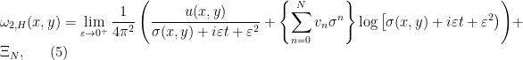
Yet, we can still have some insight into Hadamard states. A state ${\omega}$ has Hadamard form if (a) its two-point function ${\omega_{2,H}}$ has no singularities at spacelike separations, (b) for every ${N}$ , it acquires the following form in a convex neighbourhood of the spacetime ${M}$

$\displaystyle \omega_{2,H}(x,y)=\lim_{\varepsilon\rightarrow 0^+}\frac{1}{4\pi^2}\left(\frac{u(x,y)}{\sigma(x,y)+ i\varepsilon t+\varepsilon^2}+\left\{\sum_{n=0}^Nv_n\sigma^n\right\}\log\left[\sigma(x,y)+i\varepsilon t+\varepsilon^2\right)\right)+\Xi_N, \ \ \ \ \ (5)$

where ${\Xi_N\in C^\infty (M)}$ , a state that has the Hadamard form is said to be a Hadamard state. The term in parentheses is fixed by the local geometry, while ${\Xi_N}$ depends on the particular choice of state. (This is why it is better to think of Hadamard states as a class, rather than a particular state.) From (5) it is clear that if ${\omega}$ satisfies the Hadamard condition, then it must have the same singular structure as the vacuum in Minkowski. Because of this, Wick’s theorem is valid and will provide a well-defined perturbation theory.

In addition to this, the Hadamard form is of special importance when considering physical states of quantum fields in curved spacetimes. Remember that the vacuum state is that of maximal symmetry and minimum energy. Since in a generic spacetime, there are no symmetries (besides the trivial ones), there is not an obvious choice of the vacuum state anymore. As Hadamard states are well-behaved at high energies and Minkowski’s vacuum is a particular case of them, we choose them as generalizations of the vacuum. There are many examples of Hadamard states, amongst them we find all vacuum and thermal states on ultrastatic spacetimes and asymptotic vacuum and thermal states in FLRW spacetimes.

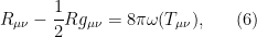
Finally, let us make a note of the importance of having a well-defined notion of objects such as ${ :\phi(x)^2:}$ in curved spacetimes. Consider the semi-classical Einstein Field Equations (sEFE):

$\displaystyle R_{\mu\nu}-\frac{1}{2}Rg_{\mu\nu}=8\pi\omega(T_{\mu\nu}), \ \ \ \ \ (6)$

where ${\omega(T_{\mu\nu})}$ is the expectation value of the stress-energy tensor with respect of the state ${\omega}$ . Recall that ${T_{\mu\nu}}$ is a monomial on the field ${\phi}$ and its derivatives. And so, terms like ${:\phi(x)^2:}$ are to be expected (this in particular, is the mass term in the free theory). It can be shown that if ${\omega}$ satisfies the Hadamard condition, then ${\omega(T_{\mu\nu})}$ will be automatically regularised. This means that the sEFE for a Hadamard state are a well-posed problem and hence in this context we will be able to study quantum fields propagating in curved spacetime.

This is all for now, in the next entry of this series I will go into the microlocal reformulation of Hadamard states, which is very elegant and powerful. Hope you enjoyed this entry!