An introduction to Conformal Welding

Here we discuss the subject of Conformal Welding, the best resource on this is given by Sharon and Mumford in a paper titled “2D-Shape Analysis Using Conformal Mapping”, I will cover some of the material that is in that paper but it will be refined for my specific interest.

As mentioned in my previous blog post, my interest lies with calculating the probability distribution of the stress energy tensor ${T}$ smeared against some real test function ${g}$ in the vacuum state. We define a test function on the circle ${S}$ to be ${f\in C^{\infty}(S)}$ satisfying certain reality conditions. We assume that our test function has support within an interval of ${S}$ . Using the definitions of state probability from the last post we can relate the Fourier transform of the probability measure to the stress energy tensor in the following way,

$\displaystyle \int_{\mathbb{R}}e^{it\lambda}dp(\lambda)=\langle e^{itT(f)} \rangle. \ \ \ \ \ (1)$

This then transforms the problem of finding the probability distribution to finding this expectation value and then inverting the Fourier transform. To get to this expectation value we will be making use of the method of conformal welding which I will now clumsily introduce.

We use the Riemann sphere ${\tilde{\mathbb{ C}}=\mathbb{C}\cup {\infty}}$ and define the unit disk as ${\Delta_{-}}$ and the complement of this region to be ${\Delta_{+}}$ . Basically just remember I’ll use a subscript minus if I’m within the region or a plus if I’m outside of it. Notice the identification between the two regions by changing the coordinates to be their reciprocal.

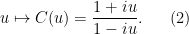
It would be reasonable to ask why we are doing all this on the circle when typically we would be interested in phenomena on the real line. I would ask you to read once more my initial post to remind yourself that we can use a Cayley map to go between the line and the circle. This mapping, for some ${u\in \mathbb{R}}$ is defined as

$\displaystyle u\mapsto C(u)= \frac{1+iu}{1-iu}. \ \ \ \ \ (2)$

If I use independent letters to denote our test functions, on the circle as ${f}$ and the line as ${g}$ . Both smooth and ${g}$ decaying at infinity, we can then relate these via

$\displaystyle f(z)=C^{\prime}(C^{-1}(z))g(C^{-1}(z)). \ \ \ \ \ (3)$

${z}$ here is on the circle, hence the argument of the test function on the real line taking the inverse Cayley transform in its argument. The observant among you may have noticed that this map is a specific example of a Moebius transform, well done you. Enough on Cayley maps for now, we return to Riemann sphere eager to see where this is going…

In ${\mathbb{C}}$ , if we take any simple closed curve ${\Gamma}$ and take its union with the region it encloses and call it ${\Gamma_{-}}$ and then the complement ${\Gamma_{+}}$ . We can then use the Riemann mapping theorem to show that there must be a conformal map between ${\Delta_{-}}$ and ${\Gamma_{-}}$ , this map is unique up to Moebius transforms. As mentioned earlier we can draw a comparison between the inside of the disk as well as the outside. The same can be said for ${\Gamma_{\pm}}$ , we use a similar coordinate transform and can then find a map between ${\Delta_{+}}$ and ${\Gamma_{+}}$ . This conformal transform is also unique up to Moebius transformations but as detailed in Sharon and Mumford, one can take a unique Moebius map such that replacing the conformal map with one composed with this Moebius transform also carries ${\infty}$ to itself and its differential carries the positive real axis of the ${\Delta}$ -plane at ${\infty}$ to the real positive axis of the ${\Gamma}$ -plane at ${\infty}$ . This eliminates the Moebius ambiguity of the external conformal map making it unique.

To cut a long story short and clarify what on earth the previous paragraph was aiming to convey. We can find the maps

$\displaystyle \vartheta_{\pm}:\Delta_{\pm}\rightarrow\Gamma_{\pm}, \ \ \ \ \ (4)$

relating the unit disk with any simple closed curves in the complex plane. Conformal welding wishes to find the map given by

$\displaystyle \varphi=\vartheta^{-1}_{+}\circ\vartheta_{-}, \ \ \ \ \ (5)$

one can think of it as a matching condition between the internal and external regions. This ${\vartheta}$ is defined on the unit circle and is a periodic real valued function with positive derivative everywhere. In my next post I will demonstrate how one can calculate these functions and then use it to find the probability distributions I am interested in.

Share this:

Like this:

Related

Leave a Reply Cancel reply