The mathematics of weather prediction and why complaining about it won’t help

Welcome back to the blog, I am taking a break from talking about conformal field theories to rant (non-seriously, I’m too apathetic to actually care) about weather prediction. Specifically I would like to discuss the challenges we face when trying to accurately calculate long term weather forecasts.

For far too long I’ve heard complaints about how “the forecast got it wrong again”, perhaps this behaviour is unique to Brits due to our proclivity for below average weather (and incessant moaning) but I somehow doubt that. This vapid whining brings disrespect to hard-working meteorological heroes ensuring that key parts of our society are able to best function in the face of challenging weather conditions with adequate preparation.

Levity aside I do feel that meteorologists get a bad rap for the hard work that they do so well, I would like to present some of the mathematics behind weather prediction in this post and then in subsequent posts I will discuss the application and some of the physical challenges which heavily impact the accuracy of these predictions (fear not, any mention of actual physical experiment will be brief and likely ill informed).

Necessary mathematical background

I’ll begin by discussing the mathematics of the system to motivate the physical requirements and limitations faced in current weather prediction technologies. If we define a fluid as a continuum of viscous deformable mass under applied shear stress or external force we can describe the motion of a fluid in a rotating pressurised gravitational field by

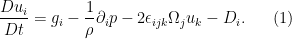
$\displaystyle \frac{Du_{i}}{Dt}=g_{i}-\frac{1}{\rho}\partial _{i}p - 2\epsilon_{ijk}\Omega_{j}u_{k}-D_{i}. \ \ \ \ \ (1)$

We have chosen to look at the ${i}$ ‘th term of this vectorial differential equation.

${\frac{D}{Dt}}$ – The “material” or “Lagrangian” derivative, equivalent to ${\frac{\partial}{\partial t} + u_{j}\partial_{j}}$
${u_{i}}$ – an element of the velocity vector of the fluid
${g_{i}}$ – an element of the gravitational field vector
${\partial_{i}}$ – an element of the gradient differential operator
${\rho}$ – density of the fluid
${p}$ – pressure
${2}$ – Just the number 2, I believe this to be equivalent to ${1+1}$ but I’d have to check with Andrew
${\epsilon_{ijk}}$ – Levi-Civita tensor
${\Omega_{i}}$ – component of the Earth’s angular velocity
${D_{i}}$ – an element of the drag force

If it wasn’t abundantly clear, I am (and will be) using summation notation, if you missed this then I suggest you revisit your old undergraduate texts!

The rotational term has come into play due to the rotating frame in which we reside. It is a mathematical description of the Coriolis effect which may be familiar to you. The drag force is assumed to be associated with the stress tensor of the fluid (order 2), the radial term is unique in the sense that it obeys, to reasonable order, ${Dw/Dt=0}$ , using ${w}$ to denote the radial component of the velocity vector in spherical coordinates.

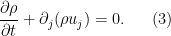
These momentum equations alone are not enough to describe the motion of the fluid, we also need a continuity equation to ensure that we aren’t creating or destroying matter. This is given as

$\displaystyle \frac{D\rho}{Dt} +\rho\partial_{j}u_{j}=0, \ \ \ \ \ (2)$

or equivalently (and in my experience more commonly)

$\displaystyle \frac{\partial \rho}{\partial t}+\partial_{j}(\rho u_{j})=0. \ \ \ \ \ (3)$

If you have never seen (1) and (3) before, don’t be fooled by the simplicity with which they have been written. This set of equations is devilishly challenging to solve, even in the some of the most basic cases. If I needed more justification for my claim, there is a Millennium prize for proving the global existence and smoothness of the solutions (or conversely that the solutions do not exist globally and that the equations break down).

In mathematical physics we love conserved quantities, they make our problems manageable. Here we have an equation for conservation of momentum, one for mass and we also are going to want to conserve energy because that seems like the right sort of thing to do. If your name is Albert you may argue that conservation of one implies conservation of all, you’re not wrong but we are assuming below light speed fluid dynamics here and we need as much help as we can get. Our energy equation will be related to temperature and I will represent it in a way to try to give as much insight into our problem as possible

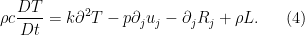
$\displaystyle \rho c \frac{DT}{Dt}=k\partial^{2}T-p\partial_{j}u_{j}-\partial_{j}R_{j}+\rho L. \ \ \ \ \ (4)$

You may recall the heat equation from an undergraduate course on partial differential equations. It is a simple, analytically solvable equation given by

$\displaystyle \frac{\partial\eta}{\partial_t}=\kappa \partial^{2}\eta, \ \ \ \ \ (5)$

where I have chosen ${\kappa}$ to deal with all of the pesky constant terms. This can be seen in (4) if one uses the alternative formulation of the material derivative applied to ${T}$ paired with the Laplacian term on the right hand side of (4).

One could group some terms by considering the flux of heat, including the radiation term ${R_{i}}$ and the diffusion term ${k\partial_{i}T}$ . This leaves us with two terms, one related to adiabatic heating from volume changes ${p\partial_{j}u_{j}}$ and latent heat exchange per unit mass ${L}$ . The constants ${c}$ and ${k}$ are simply the specific heat capacity of the fluid and diffusion coefficient respectively but they are constants so who really cares, I could always just set them to 1.

The group of equations (1), (3) and (4) together are known as the Primitive equations. These five equations have five unknowns ${(u,v,w)}$ , ${p}$ and ${T}$ giving theoretically, the ability to be able to solve these equations. Anyone reading this who has worked with partial differential equations may have the inclination that it is not quite as simple as that. I’ll leave it here today, next time I’m planning on briefly discussing solutions of general partial differential equations, application of those ideas to the Primitive equations and then finally motivate physical limitations of our idealised problem. If you only take away one thing let it be this, weather dynamics follows the laws of fluid mechanics and energy conservation.

Share this:

Like this:

Related

Leave a Reply Cancel reply